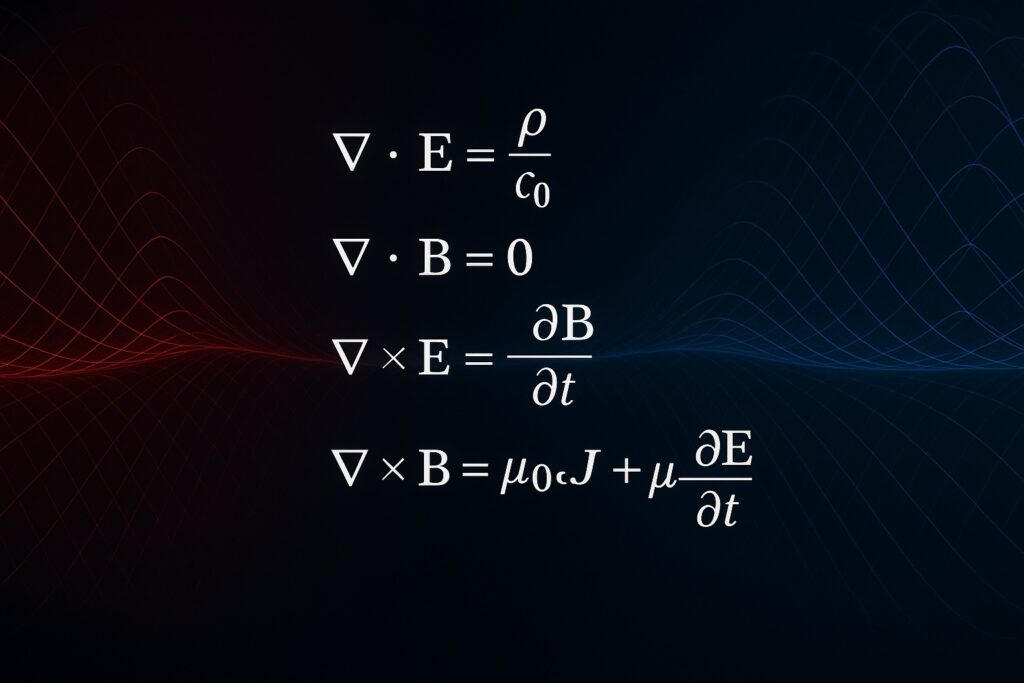
Maxwell’s equations are the cornerstone of classical electromagnetism, unifying the previously distinct fields of electricity, magnetism, and light into a single, simple set of four equations. This unassuming set of equations stands as arguably the most important physics discovery of the 19th century, providing engineers across the globe with the theoretical basis for understanding the behavior of electromagnetic waves. Consequently, nearly all electronic devices we use today, from antennas and electric cars to the humble toaster, have almost certainly been designed and optimised using principles laid out by Maxwell’s equations.
My goal for this project is to gain an intuitive and mathematical understanding of the fundamental principles that govern our modern world of electronics and communication, which is not provided by the A level course (at the time of writing I have completed only first year content). The article will go law by law providing an explanation for what each equation states and deriving them not using calculus but rather through more conceptual and intuitive explanations of the divergence and curl of electric and magnetic fields.
Gauss’s Electric Law
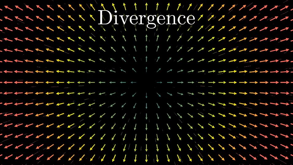
To understand Gauss’s Law in its differential form, it is helpful to conceptualize the electric field, E, as a vector flow field in space. The mathematical operation known as divergence, denoted ∇, defines the behavior of this field (E) at any specific point in the field. A positive divergence at a point signifies a source, indicating a net outflow from an infinitesimal region surrounding the point. Conversely, a negative divergence signifies a sink, indicating a net inflow into such a region. If the divergence is zero, there is no net origination or termination of field lines within the region; the flow merely passes through.
The sources or sinks of this electric field are identified as electric charges in Gauss’s first law. By convention positive electric charges function as sources, from which electric field lines originate and extend outward. The magnitude of this source effect is proportional to the charge density, ρ, within a given region. Negative electric charges, conversely, function as sinks, towards which electric field lines converge. Similarly, the magnitude of this sink effect is determined by the density of negative charge.
This local relationship between field divergence and charge distribution is precisely formulated by Gauss’s Law in its differential form:
$\Delta \cdot E = \frac{\rho}{\epsilon _0}$
This equation states that the divergence of the electric field (∇⋅E) at any point is directly proportional to the electric charge density (ρ) at that same point. The constant $\epsilon _0$, the permittivity of free space, is a fundamental physical constant that ensures both dimensional consistency and quantifies that if electric fields travel through mediums of high “resistance” to electric fields the magnitude of the vectors must decreases.
Gauss’s Magnetic Law

The magnetic field, denoted as B in Maxwell’s equations, can also be conceptualised as a vector flow field in space. Its divergence, ∇⋅B, quantifies any net outflow or inflow from a point. Gauss’s Law for Magnetism, a fundamental principle of electromagnetism and one of Maxwell’s equations, states that this divergence is universally zero:
$\Delta \cdot B = 0$.
This means that the net magnetic flow is always zero and magnetic fields must form closed loops, with all field vectors eventually returning to their origin. Consequently, distinct absence of origination and termination points cannot exist under Gauss’s second law meaning that magnetic monopoles are physically impossible - in contrast to the electric field.
It is noteworthy that no fundamental principle actualy forbids magnetic monopoles, and some advanced theories like string theory even predict their existence. These theories suggest their predicted properties, such as extreme mass and high-energy formation requirements, could explain their current elusiveness. Consequently, the search for magnetic monopoles remains an active area of physics.
Faraday’s law
Next, we turn to Faraday’s Law of Induction, a discovery that unveiled a profound connection between magnetism and electricity, showing they weren’t just static partners but could dynamically influence one another leading to the vital creation of the generator - an invention used ubiquotiously in the national grid.
Michael Faraday, through meticulous experimentation, demonstrated that a changing magnetic environment could induce an electromotive force (EMF), a force that drives current through a conductor. The core concept in the induction of EMF revolves around “magnetic flux” (Φ), which quantifies the amount of magnetic field lines piercing a given area. Faraday’s Law states that the induced EMF (ε) in any closed circuit is proportional to the rate of change of the magnetic flux through that circuit or how many magnetic field lines are piercing area per second:
$\mathcal{E} = -\frac{d\Phi_B}{dt}$
The minus sign, a crucial addition known as Lenz’s Law, signifies that the induced EMF (and any resulting current) will always act to oppose the change in magnetic flux that produced it – to adhere to the conservation of energy stopping an otherwise infinite propogation of electric and magnetic fields.
Feynman further clarifies that this change in magnetic flux can occur in several ways: the strength of the magnetic field (B) itself can vary over time, the area (A) of the loop through which the field passes can change, or the orientation of the loop relative to the field can alter. Regardless of the specific mechanism, if the total magnetic flux is changing, an electric field must be generated. This electric field differs from the divergent electric fields produced by static charges (as described by Gauss’s Law); rather, as Feynman notes, it’s an electric field that forms closed loops, a “curly” electric field. This “induced” electric field is what exerts a force on charges within a conductor, giving rise to the EMF.
Maxwell translated Faraday’s integral law into its more local, differential form:
$\nabla \times \mathbf{E} = -\frac{\partial \mathbf{B}}{\partial t}$
This compact equation elegantly states that a time-varying magnetic field (∂B/∂t) will always be accompanied by a spatially varying, circulating electric field (realised through the mathematical operator ∇ × E, which represents the “curl” of E). It was no longer just about wires and magnets; but rather a fundamental property of the fields themselves. This equation, paired with Ampère’s Law (which we’ll explore next, along with Maxwell’s crucial addition to it), reveals how changing electric and magnetic fields can generate each other, paving the way for the understanding of electromagnetic waves, and ultimately, light itself.
Ampere-Maxwell law

A fisherman using the Ampere-Maxwell law (electromagnetism) to retrieve an old car
The fourth and final cornerstone of this electromagnetic edifice is the Ampere-Maxwell Law and arguably the most important law in our modern world, describing the production of magnetic fields from electric currents. This concept is essential in speakers, motors and electromagnets - some of the most prevalent technology on earth.
The original Ampere law stated that magnetic fields (denoted as B) would “circulate” or “curl” around electric currents producing a magnetic field. Mathematically, in its differential form, this was expressed as;
$\nabla \times \mathbf{B} = \mu_0\mathbf{J}$
where J is the electric current density and μ₀ is the permeability of free space.
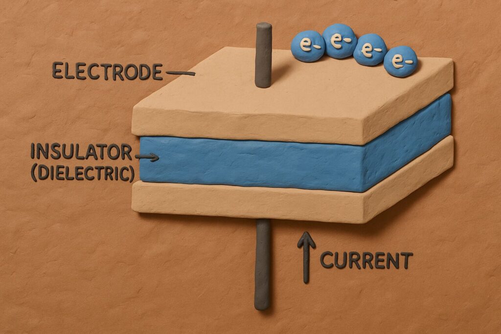
This law worked beautifully for steady currents, such as those flowing continuously in wires. However, James Clerk Maxwell identified a critical flaw when applying it to situations with changing electric fields. A key example is the space between the plates of a charging capacitor, where the capacitor is charged through the charging of plates with no actual current flow. Despite no current passing through the capacitor, a magnetic field is still observed around this gap—a phenomenon Ampere’s original law was unequipped to explain and suggesting the electric field between the charges may induce a magnetic field.
To address this inconsistency Maxwell proposed an additional source term for magnetic fields: a changing electric field. He introduced what he called the “displacement current” density
$\mathbf{J}_D = \epsilon_0 \frac{\partial \mathbf{E}}{\partial t}$
, where ε₀ is the permittivity of free space and ∂E/∂t is the rate of change of the electric field (relative to time).
As Feynmann clarifies, this new term; “displacement current” is crucially not a flow of charge in the traditional sense, but it acts just like a real current in its ability to produce a magnetic field. By adding this term, Maxwell not only resolved the inconsistency seen in the capacitor example but also completed the symmetry between electricity and magnetism. If a changing magnetic field could induce an electric field (by Faraday’s Law), then a changing electric field should, in turn, induce a magnetic field.
Thus, the complete Ampere-Maxwell Law became:
$\nabla \times \mathbf{B} = \mu_0\mathbf{J} + mu_0\epsilon_0\frac{\partial\mathbf{E}}{\partial t}$
This equation now states that a magnetic field can be generated by two means: by actual electric currents (μ₀J) or by a time-varying electric field (μ₀ε₀∂E/∂t).
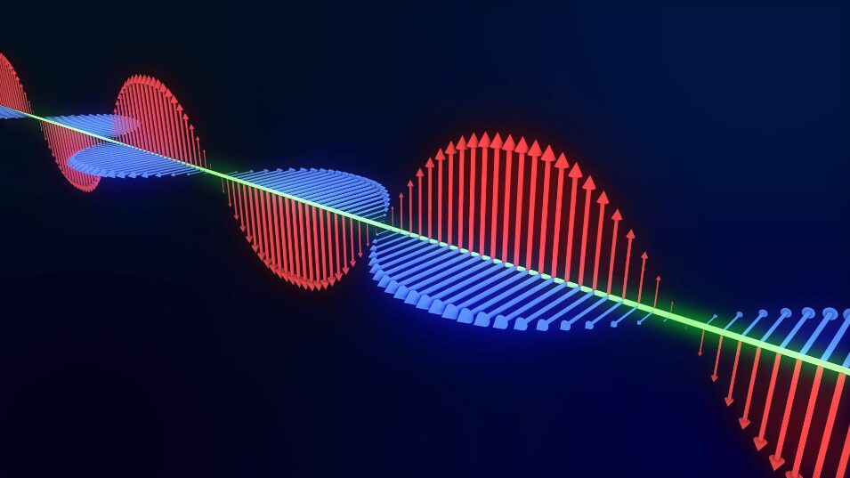
While this addition may just seem like a simple corrrection it was the key that transformed our understanding. With Faraday’s Law showing that changing magnetic fields create electric fields, and the Ampere-Maxwell Law now showing that changing electric fields create magnetic fields, the stage was set for a brilliant realisation. These two laws together described a self-sustaining dance: a changing electric field generates a changing magnetic field, which in turn generates a new changing electric field, and so on. This interplay allows for the propagation of electromagnetic waves through space, even in a vacuum devoid of charges or currents. Maxwell had found the mechanism for light.
Conclusion
This project article, aimed at intuitively understanding Maxwell’s equations beyond A-level, has been a profound journey for me from Gauss’s laws on field sources, through Faraday’s dynamic induction, to the critical completion of Ampere’s law by Maxwell. The true marvel emerged in seeing how these laws interlink, revealing the elegant self-sustaining dance of changing electric and magnetic fields that birth electromagnetic waves—and thus, light. This exploration has solidified not just the individual importance of each equation, but their collective power in redefining our universe and underpinning modern technology.